Neural networks are one of the biggest innovations in artificial intelligence (AI), and the driving force behind the recent excitement in the field. However, to truly understand neural networks, we need to go back to the 1940s, when the perceptron was invented.

Perceptrons are a type of linear binary classifier—they can only separate data into two categories—and they belong to the supervised learning family of algorithms. If you’re unfamiliar with these terms, be sure to check out our introductory article on machine learning.

Understanding the perceptron is the first step in grasping the mechanics of neural networks. In this article, we’ll explain what perceptrons are, how they work, their limitations, and their history.

What are Perceptrons?

If neural networks can be likened to a biological brain, a perceptron is comparable to a single neuron. Much like neurons, perceptrons receive information, process it, and, depending on the outcome, decide whether or not to generate an output signal.

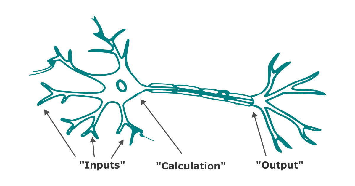
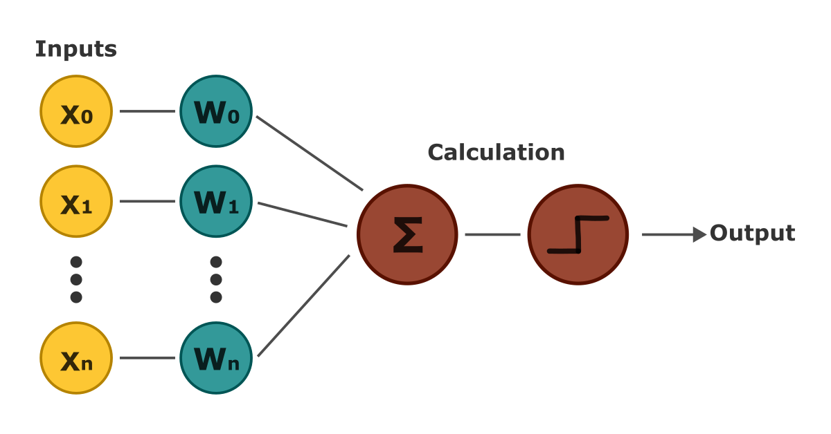
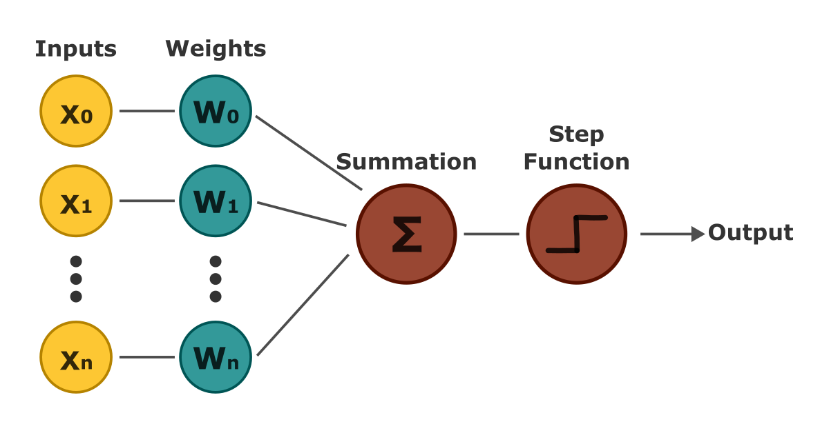
Perceptrons consist of four main components: the inputs (our data), weights assigned to the inputs, a bias term, and the Heaviside step function—a function that returns 1 for positive inputs and 0 for negative ones.

The inputs are multiplied by their corresponding weights, and the bias is added to the result. This value is then passed through the Heaviside step function, h(x), which outputs either 1 or 0. Mathematically, the output of a perceptron can be represented as follows:

As the formula shows, the perceptron defines a linear relationship between inputs and outputs, making it a linear classifier. Because the step function outputs only 1 or 0, a single perceptron can only classify binary data.

We can simplify the equation by merging the weights with the bias by adding an extra dimension of 1’s to the inputs. This adjustment is mathematically equivalent to the original, but it simplifies the training process for the bias term. Visually, our final perceptron would follow this diagram:

Before diving into the learning algorithm, let’s clear up a potential point of confusion. In the diagram, each input point represents a dimension of input data, not individual data points. The number of weights corresponds to the number of features, not the quantity of data.

For example, if we have data on eye and hair color from 1,000 people, there are only two features (eye color and hair color), so the perceptron would have two weights and a bias term.

How do Perceptrons learn?

Having a linear function between inputs and outputs doesn’t achieve much by itself if we don’t know the weights. This is why perceptrons require training. We can adapt the gradient descent algorithm to train perceptrons to learn the appropriate weights. If you’d like a more detailed explanation of gradient descent, you can read this article.

Unlike raw gradient descent, we can’t follow the gradient here, as the step function has a gradient of zero. Instead, we look at the difference between the expected and predicted outputs and update the weights only if the prediction is incorrect. This is achieved by the 0-1 loss function.

Loss functions could be an entire topic on their own, so for now, we’ll focus on the learning rule for perceptrons:

Here, w_i refers to the weights for each of the n features, d is the actual output, y is the predicted output, and t is the current iteration. Perceptron weights will only converge if the data is linearly separable.

Implementing Perceptrons with Python

Let’s actually build our perceptron in Python. We will create a class called “Perceptron” that stores the weights and bias, with functions to predict outputs and train the weights as mentioned earlier.

The initialization function will look like this:

class Perceptron:
  def __init__(self, learning_rate, weights_shape, depth_limit=1000):
    
    self.learning_rate = learning_rate
    self.depth_limit = depth_limit
    
    # Initialize the weights
    np.random.default_rng()
    self.weights = np.random.rand(*weights_shape)  # Contains the bias

It might be tempting to include input and output matrices in the perceptron class, but instead, we’ll pass the inputs directly as arguments to functions. This keeps things flexible and allows us to feed the perceptron new data easily.

Our predict function will handle the forward computation, passing the result through the Heaviside step function:

# Applies heaviside step function vector-wide
def step_function(self, inputs):
  return np.where(inputs >= 0.5, 1, 0)


# Predicts the output for a given input
def predict(self, inputs):
  return self.step_function(np.dot(inputs, self.weights).T)

The only remaining part is the training function, which we’ll split into two: train_step for a single iteration, and train to loop through until convergence. This simply makes it easier to create visualizations in case you also happen to write tutorials.

# Returns the output of a single training step
def train_step(self, inputs, outputs):
  diff = outputs - self.predict(inputs)
  self.weights = self.weights + self.learning_rate * np.dot(diff, inputs).T
  
  
# Trains the perceptron until convergence
def train(self, inputs, outputs):
  it = 0
  while it < self.depth_limit and not np.all(outputs == self.predict(inputs)):
    self.train_step(inputs, outputs)
    it += 1

That’s all we need to have a functioning perceptron. Just like that, we have technically implemented our first neural network using nothing but NumPy.

Using our Perceptron on Data

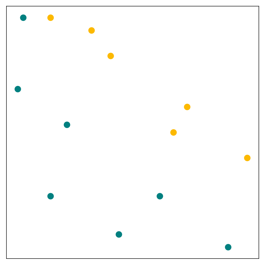
Let’s see our implementation in action. We can use any linearly separable dataset, but the Single Layer Perceptron Dataset by Abir Hasan on Kaggle is small, easy to visualize, and most importantly, in the public domain–perfect for our case. Looking at features 2 and 3, we can confirm that it is indeed linearly separable, at least along these dimensions:

We can then initialize and train our perceptron:

perceptron = Perceptron(learning_rate=0.1, weights_shape=(inputs.shape[-1], 1))
perceptron.train(inputs, outputs)

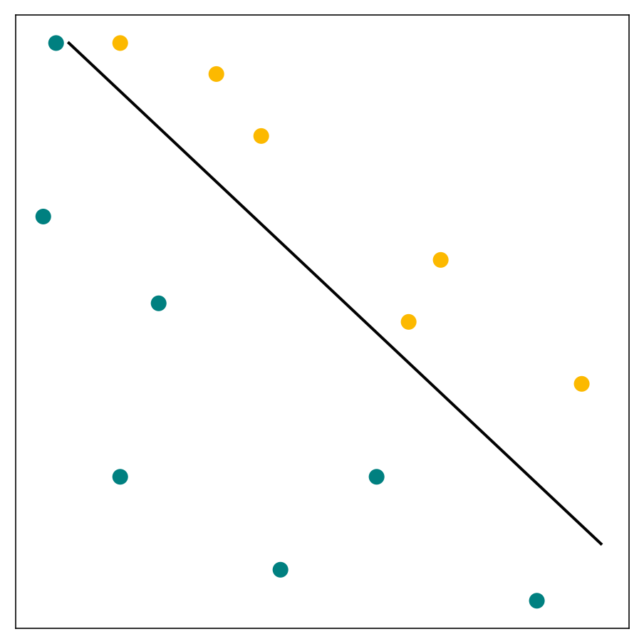
Once training converges, we’ll notice that the weights have been changed. We can visualize the line formed by these weights using pandas and matplotlib:

Limitations of Perceptrons

Despite its simplicity, a single perceptron is already a complete neural network–a feedforward neural network, to be precise. However, this doesn’t mean that a single perceptron by itself is sufficiently powerful for complex problems.

For example, although a perceptron can mimic logical functions like AND or OR, it cannot model the XOR function. This inability to solve non-linearly separable problems led to the AI winter, a period during which AI research and funding slowed significantly.

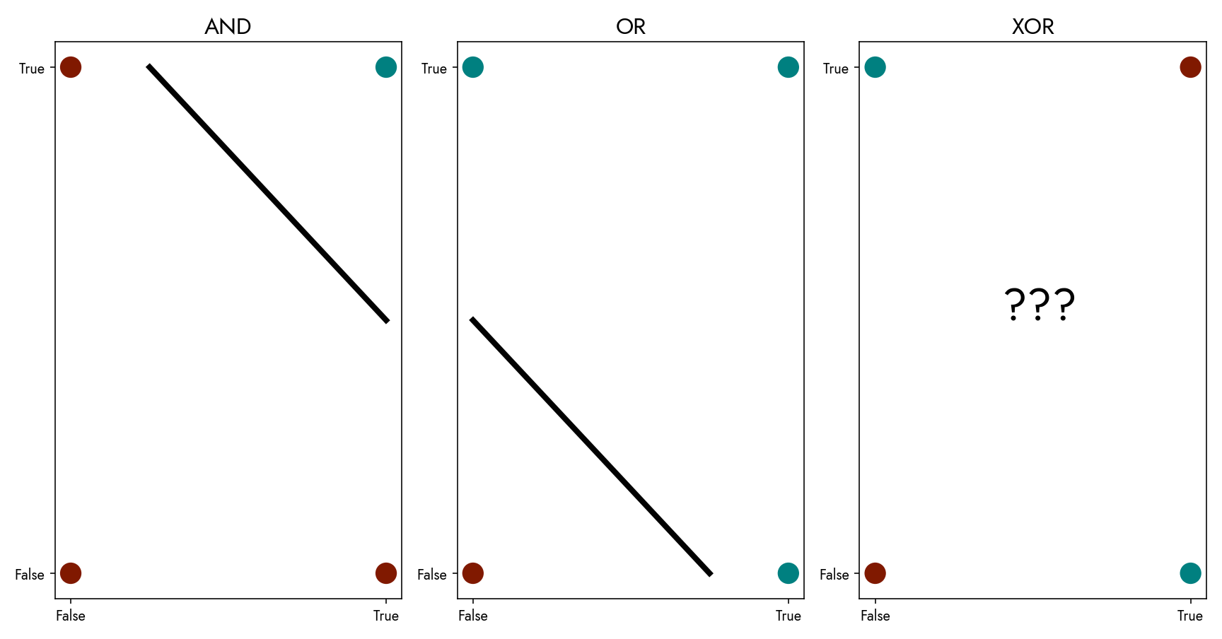
Another limitation is that perceptrons require linearly separable data to converge. If the data isn’t linearly separable, the perceptron will simply fail to find a solution.

Multilayer Perceptrons

Many of these limitations can be overcome by connecting multiple perceptrons into a network. After all, individual neurons in the brain don’t do much on their own, but together, they form complex networks. Such networks are called multilayer perceptrons.

Perceptrons naturally lend themselves to interconnectivity—one perceptron’s output can serve as another’s input. This concept is key to building neural networks and is the reason they are so powerful.

For instance, the XOR problem we mentioned earlier can be solved using multilayer perceptrons:

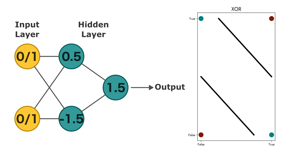
At this point, we’re only one step away from modern feedforward neural networks. The Heaviside step function we’ve been using is the main barrier because it has a zero gradient, preventing us from applying gradient-based learning methods like backpropagation.

There are other functions that offer continuous gradients for all inputs. These functions are collectively called activation functions. There are many important ones, each with its own benefits and drawbacks, which we will cover in another article.

Closing Thoughts

In this article, we explored the fundamentals of perceptrons and implemented a basic version in Python. While single perceptrons aren’t commonly used today, their invention marked a pivotal moment in AI history. Practically, they represent the simplest neural network possible, making them a great learning tool before tackling more complex models.

Next, we’ll delve into feedforward neural networks, which are the natural evolution of perceptrons. If you’d like to learn more, be sure to subscribe to our newsletter. Until then, stay curious!